Policy rate tightening
With all this talk about Fed tightening in the autumn with UK rises to follow in early 2016, it might be useful to remind ourselves of the strong inverse relationship between stir futures and policy rates. Of course, stir futures are LIBOR linked derivatives but LIBOR is very closely correlated with policy rates making stir futures ideal for the systematic trading of policy rate changes.
The first chart shows the front month continuous short sterling contact (orange RHS) and the BOE Base Rate (purple LHS) over the last 20 years.
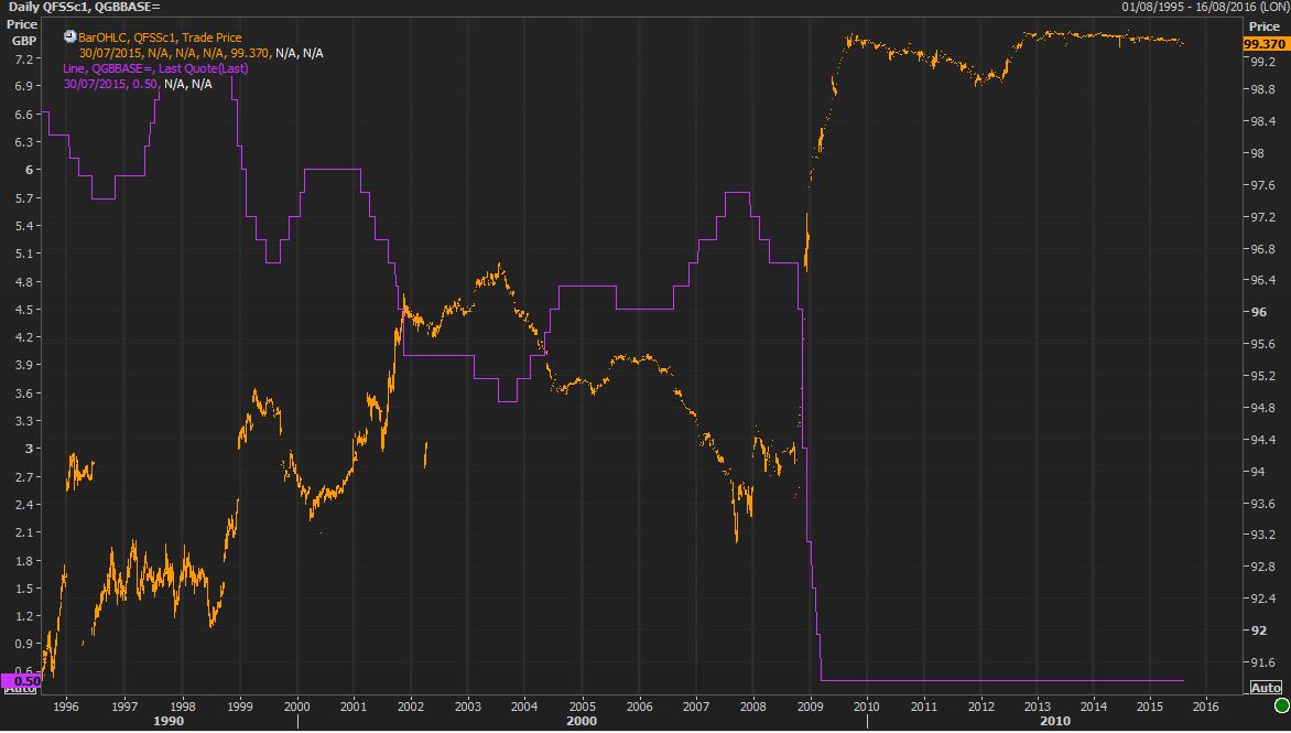 Source: Reuters Eikon
The inverse relationship is clear and most importantly shows that when policy rates start changing, stir futures start trending.
Same with the US. (Eurodollar front month continuous in purple (LHS) and Fed Funds Effective Rate in orange (RHS)
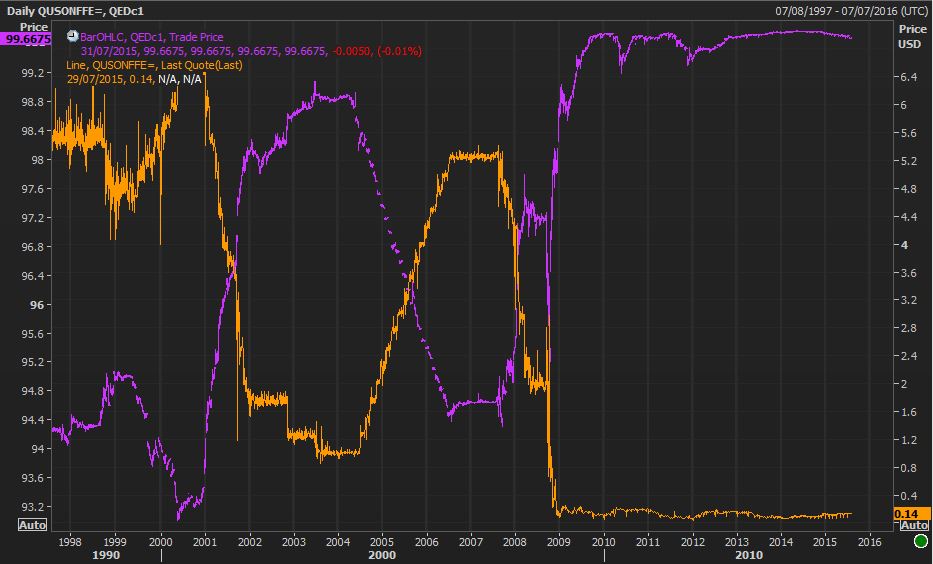
Source: Reuters Eikon
It can also be observed that the US often acts preemptively to the UK. When America sneezes, the UK catches a cold.
The year -end turn effect
The year-end effect in STIR futures is a legacy from the 1980’s. There are often high borrowing requirements at year end as Banks look to bolster their cash reserves at the end of a fiscal year or quarterly period. This requirement and the fact that the days straddling the end of one year and the beginning of the next fall in the holiday season and create an overnight borrowing period that can be two or four days in duration due to bank holidays.
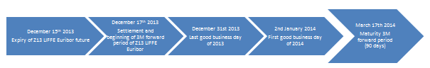
In December 2013, the year end turn effect would have been muted since money could have been borrowed on Tuesday 31st December 2013 and returned on Thursday 2nd January 2014. This would have been just two days but if those days had straddled a weekend, it could have been four. It can have an effect on STIR futures because year end is included in the forward period covered by the December contract.
If the forward deposit period rate was 1%, then the futures implied rate should be
However, if rates jumped to 1.5% over the turn, the futures implied rate would be:
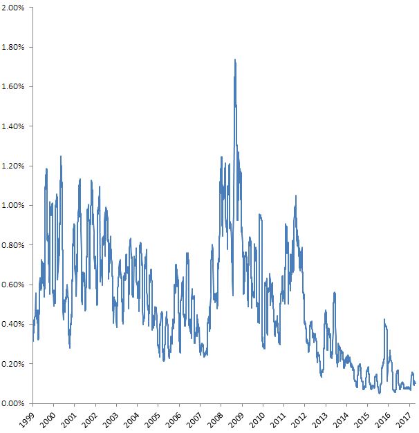
Clearly this is insignificant when the turn premium is 0.50% and the turn period two days so it is off most STIR trader’s radar apart from the most exceptional periods like run up to December 1999 when the markets were spooked by the millennium bug (Y2K) fears. This was most clearly observed in the Sterling Dec butterfly.
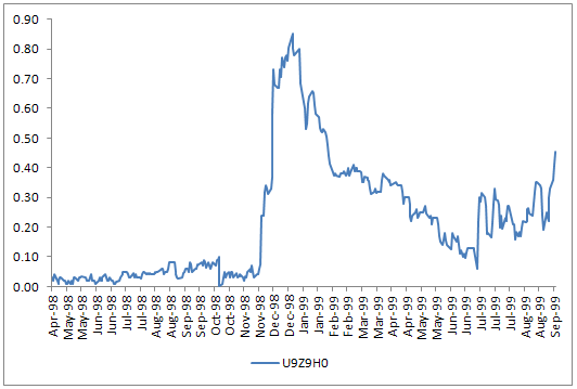
LIFFE Short Sterling U9Z9H0 butterfly Apr 98 to Sep 99 (price differential)
Worries that that non Y2K compliant Banks would be refused year end funding caused the Z99 future to fall sharply relative to the surrounding U99 and H0 contracts, causing the usually staid butterfly spread to blow out by around 80 ticks (bps). This also happened to Eurodollar and Euribor and was probably a once in a generation occurrence but watch out for potential repeats driven by, for instance, rumours of Banks failing regulatory requirements.
Looking at the latest set of Euribor Dec butterfly’s in the chart below, there are no discernible Dec premium reflecting year-end turn premiums, mainly because Central Banks are very adept at financing these days and post the financial crisis, Banks have relatively easy access to central bank funding
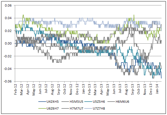
LIFFE Euribor Butterfly’s (Dec fly’s are coloured and surrounding fly’s are greyed for contrast)
However, despite the fact that the year-end turn effect seems to be diluted by the relatively small turn premiums in Dec fly’s these days, there is another aspect to consider relating to year end liquidity:
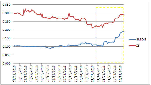
Stricter liquidity regulation caused a significant reduction in the liquidity available in the overnight market during December 2013, which fuelled sharp upward pressure on the overnight cost of cash. Having started December at 11.2bp, EONIA moved up to 20.6bp on 17 December, then declined a little to 17.1bp on 24 December before spiking in the last week of the year to 44bp in an illiquid market.
This effect can be observed on changes in the Euribor strip.
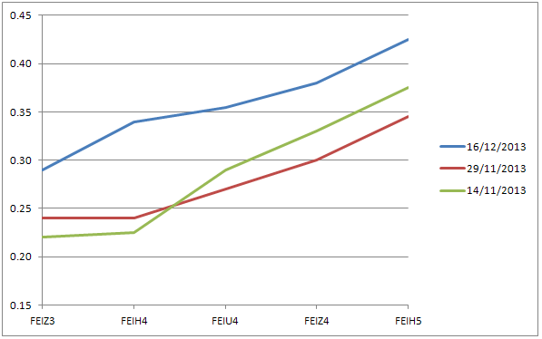
LIFFE Euribor Strips November to December 2013
The strip yield increases, almost in parallel as condition tighten in the EONIA market during December and the causal link is observable between 3M OIS and Euribor Z3.
Indeed, there seems to be a general pattern of tighter overnight rates in the euro zone and a quick study reveals that in seven out of the last ten years (2004 to 2013), Euribor futures closed lower (rates higher ) at the end of December compared to where they started December.
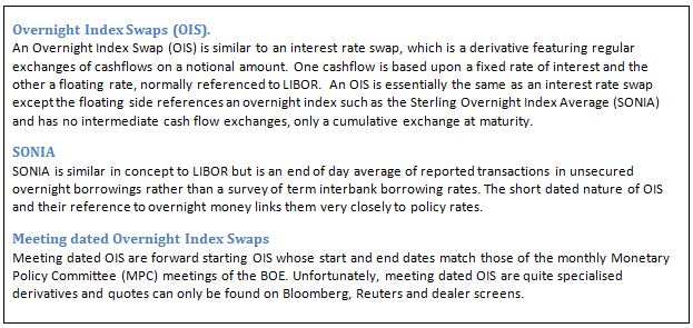
Interest rate change probabilities
STIR futures are not the ideal instrument for determining policy rate change probabilities since they are LIBOR or EURIBOR linked derivatives. These 3 month interbank fixings are not the same as policy rates and there is often substantial disparity between them. However, STIR futures are often used to speculate on or hedge against changes in official interest rates due to their liquidity and transparency since all short rate products will generally reflect changes in policy rates.
There has recently been much in the UK press about the Bank of England’s (BOE) forward guidance policy. Market expectations of base rate increases have been pulled forward in response to improving economic conditions, particularly the rapid decline in unemployment.
It is possible to determine the probabilities of base rate changes within a particular time frame by the use of a specific instrument called a Meeting Dated Overnight Index Swap.
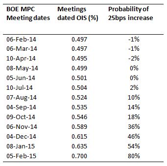
The table below shows the BOE MPC meeting dates for the next year and corresponding meeting dated OIS rates.
Example
The rate for the MPC meeting on 8th May 2014 is 0.499%. This rate is the market rate of a one month forward starting OIS, starting on 8th May and maturing on 5th June. 0.499% is the fixed OIS rate quoted against receiving compounded daily SONIA for one month between these dates. If base rates were increased on or before 8th May from the present level of 0.5% to 0.75%, then the OIS fixed payer would be in the money, paying just 0.499% for a month against receiving SONIA which would have increased to around 0.75%.
The probability of a 0.25% (25bps) increase in the base rate on or before 8th May would be calculated as:
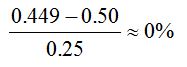
This is basically saying that the market puts 0% probability of a 25bps base rate increase occurring by May 2014. This probability has increased to 80% by February 2015 reflecting the current market consensus for the first 25bps increase in base rates to occur early in Q2 2015.
The graph below illustrates the term structures of MPC dated OIS, market consensus base rate forecast and the LIFFE Short Sterling STIR futures strip (expressed as implied forward rates).
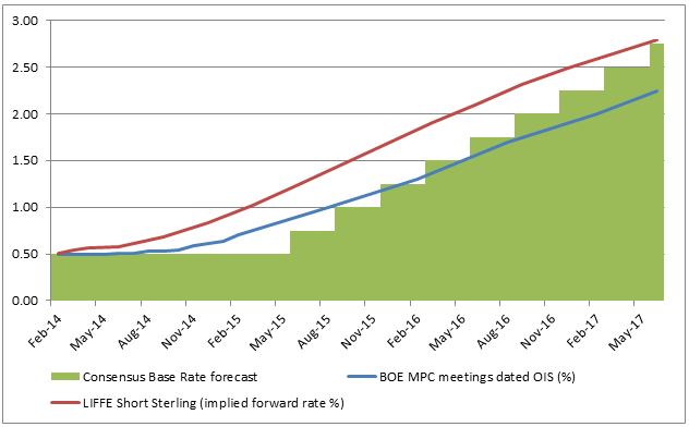
Term structures of UK BOE MPC dated OIS, market consensus UK BOE base rate forecasts and the LIFFE Short Sterling STIR futures strip (expressed as implied forward rates): Late January 2014
The Short Sterling futures should not be interpreted as being more aggressive in terms of interest rate expectations, the difference between the rates just reflecting their types: forward SONIA OIS as compared to forward 3M LIBOR. However, the gradient of the Short Sterling term structure suggests uniformity with the OIS expectations, suggesting equilibrium between products in terms of future interest rate expectations.
From a traders perspective, if rates were thought to increase sooner and faster than expected, then the curve would steepen (buy Short Sterling calendar spreads) and if rates were thought to be on hold and increase at a much slower rate than forecast, then the curve would flatten (sell Short Sterling calendar spreads). Watch this space…
Understanding open interest
Open interest (OI) is the total number of outstanding futures contracts that are not closed or delivered on a particular day. It is a useful measure of liquidity of in a futures contract and many technical practitioners consider it a useful barometer for trend detection.
The following table illustrates how open interest is determined.
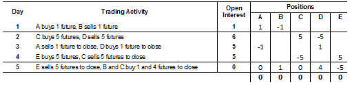
Open interest comes in two forms, individually per contract (e.g. H14) or for all contracts (e.g. all Euribor futures). The open interest for all contracts, often termed Market Open Interest is a useful barometer of liquidity and activity within a product. Technical practitioners generally expect open interest to increase when a trend is establishing and reduce when the trend is coming to an end.
The charts below shows market open interest and price (continuous) for the Eurodollar and Euribor.
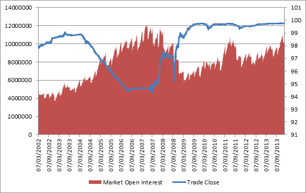
Eurodollar market open interest (LHS) and close (continuous contract) (RHS) 2002 to 2013
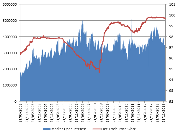
Euribor market open interest (LHS) and close (continuous contract) (RHS) 2002 to 2013
There does not seem to be an obvious link between increasing open interest and price action but it might be useful to keep a watch on contract levels to gauge any potential flows.
LIFFE’s STIR matching algorithm
Matching algorithms are the mathematical equations within the computer code of the Exchange matching engine, known as CONNECT on LIFFE. These algorithms allocate incoming market orders amongst the resting order depth using a methodology somewhere between a pure pro rata and pure time priority, also known as first in-first out (FIFO).
LIFFE operates two matching algorithms for its STIR futures: one for Euribor and the other for Short Sterling and Euroswiss. They combine both pro-rata and time priority but the Short Sterling /Swiss version has a higher bias towards time priority.
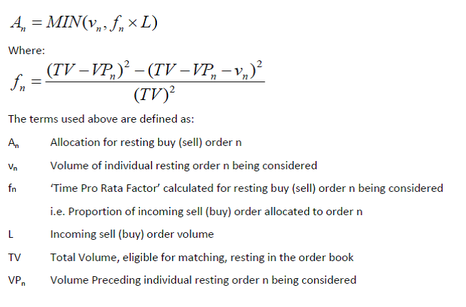
Both algorithms have the same mathematical structure. The current algorithm for the Euribor is:
The current algorithm for Short Sterling and Euroswiss is similar but to a higher order*.
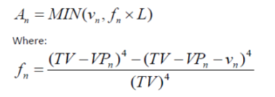
*The Time Exponent employed within the Gradual Time Based Pro Rata (GTBPR) matching algorithm will change from 4 to 2 effective on Monday 3 December 2018
An easy way to consider these algorithms is as if the order is set to 1 (i.e. there are no powers). In this case, any incoming order of reasonable size is split amongst resting orders in an equal percentage weighting.
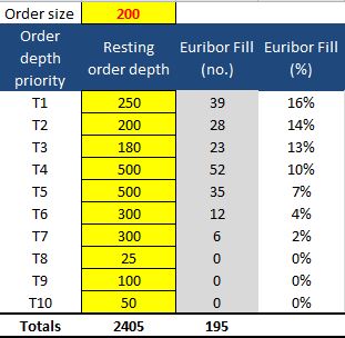
Example
The table shows an incoming order of 200 lots into a market with a resting order depth of 2405 lots made up of 10 individual orders of different size and ranked by time priority. It could be considered as a market order to sell 200 lots at best when the market is 99.00 bid for 2405 lots. The 2405 lots on the bid are made up of 10 separate orders all bidding the same price but entered at different times. The order with the oldest timestamp will be T1 and the newest T10.
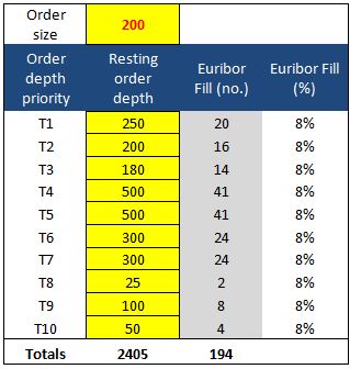
It can be seen that all orders (T1 through to T10) get 8% of their resting order size. In absolute terms, the larger the bid, the more futures would have been bought. It might be noted that only 194 futures were transacted and so the algorithm would then make another pass to allocate the remaining 6.
This is an example of pure pro rata and would advantage those over quoting by flashing large orders into the market depth momentarily before the order hits the market and would provide no advantage to consistent resting liquidity providers. To circumvent this, the actual algorithms operate to a power; two in the case of Euribor and four in the case of Short Sterling and Euroswiss.
The same order and market depth then experiences a very different allocation. The Euribor algorithm allocates on a broadly linear but decreasing profile (in percentage terms) whereas the Sterling/Swiss algorithm would allocate a much higher proportion to the first three time priority orders (T1-T3) with sharply decreasing density thereafter for the remainder. In both cases, orders towards the back of the queue get no allocations.
In graphical terms the effect is more observable.
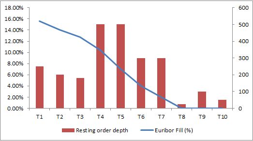
Both algorithms, but particularly the Sterling one, benefit orders with time priority; the idea being to promote and encourage resting liquidity. Traders are encouraged to supply liquidity early into price points.
The spreadsheet containing both algorithms is available to download here. Now you can figure out for yourself why your fills might not be what you hoped for and perhaps find a way to improve your allocations.
Bund rolls
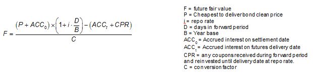
Bund futures are complicated by their contract design which stipulates physical delivery by the Short for each futures contract of €100,000 face value from a choice of deliverable bonds. Conversion factors exist to compensate for a bond being delivered with a coupon other than the 6% also specified in the contract design. This process involves the Long paying the Bund EDSP x the conversion factor + Accrued Interest on the delivery date on the bond being delivered and gives rise to cheapest-to-deliver optionality, when the yield curve is anything but 6%.
The theoretical value of the Bund future should be the forward value on the delivery date of the cheapest to deliver in the basket of deliverable bonds, divided by the conversion factor.
Unfortunately, that’s not the end of the story, rather the start. If you were to price a bund future using the above formula you would find it was higher than the actual market price of the future. This is the net basis (when multiplied by the conversion factor) and reflects all that embedded optionality mentioned above. The optionality exists because the cheapest to deliver bond underlying the bond future can change plus there are additional sources of optionality; namely switch and wildcard optionality, which are specific to the actual delivery process.
All the above are known knowns and have been for over two decades. Consequently, that means that the embedded optionality in bund futures is pretty fairly quantified by the market, leaving things like bund rolls being driven by more mundane things like supply and demand and financing considerations. Bund rolls are the effect on the calendar spread of the rolling process of open positions in the front month into the back month to maintain directional bias.
The chart shows the effects of the Z3H4 roll. The blue and red shading is open interest for Z3 and H4 respectively (left axis) and the Z3 and H4 prices are prices on the right axis.
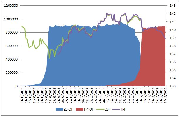
It can be seen that the open interest in Z3 coincides with a rally in Z3 bund prices and so it could be inferred the trend following traders, (systematic hedge funds like MAN, Winton and Bluetrend plus CTA’s) are long and might want to maintain the positions into H4. This means at some stage they will have to sell their Z3 holdings and buy H4 futures. This would cause a spread cheapening or narrowing. The window for trading the roll is quite narrow since it can be seen that the H4 doesn’t come to life in trading volume or OI until early November 2013, and doesn’t really pick up until end of November. This means that there is only about two weeks in which to actively trade the roll but the trader could have actively positioned expecting a roll of long interest by selling the Z3H4 spread.
The following chart shows that the Z3H4 spread could have been sold in early November for around zero and subsequently fell about 15 ticks by early December. Only in the last days did the spread widen dramatically.
Bund rolls are amazingly complex driven by a multiple of factors.
- Embedded optionality considerations
- Relative value of each futures contract to the basket of underlying deliverable bonds.
- Changes in bond financing rates (repo)
- Directional bias of open interest.
Often it is changes in repo rates that can cause volatility in the final days approaching the last trading day of 6th December. Bunds that are cheapest to deliver can often trade special, sometimes at negative repo rates which can make the futures contracts drop. That might have happened here to the H4 relative to the Z3.
The disappearing convexity bias
The convexity bias is a technical trade-off between either a strip of STIR futures versus an interest rate swap, or in single period terms, a trade off between a single STIR future and an equivalent term forward rate agreement (FRA). A FRA is an over-the-counter bilateral product that allows the buyer /seller to notionally borrow/lend a specified amount at a LIBOR linked rate over a forward period.
What is the convexity bias?
The rationale for the convexity bias exists due to the FRA’s convex payoff compared to STIR futures linear payoff. As underlying rates move up and down, a position in STIR futures will have the same payoff but that of the FRA will change. The convexity of the FRA comes about due to its discounted payoff.
- The payoff of a short STIR future is given by (L%-F%)* 10000*$25
- The payoff of a short FRA is given by ((F%-L%)* Notional*0.25)/(1+L%*0.25)
Where
- F% is the FRA forward rate or rate implied by STIR
- L% is the FRA maturity date LIBOR rate or futures EDSP rate.
- 0.25 is the 3-month accrual (in reality measured by ACT/360 convention for USD and EUR)
- $25 assumes Eurodollar tick value per basis point.
Example:
The table shows the convexity bias between a position of short 1000 Eurodollar (ED) futures and an offsetting short $1005m 3-month FRA (slightly more than $1000m to compensate for discounting methodology), both instigated at a rate of 2%.
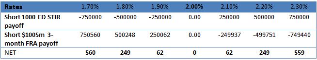
- An increase in underlying rates from 2% to 2.10% would result in a credit to the variation margin account of short 1000 ED STIR position of $250,000 and a debit of slightly less than that in the discounted equivalent of $1005m 3M FRA collateral account (assuming zero threshold – zero threshold means every dollar of value change has to be made good.).
- A decrease in underlying rates of 10 basis points to 1.9% would result in a debit to the variation margin account of a short 1000 ED STIR position of $250,000 and a credit of slightly more than that in the $1005m 3-month FRA collateral account (assuming zero threshold).
If the rates on both products were the same, there would be an advantage or bias in borrowing (selling) via the STIR future and lending via a short FRA to take advantage of the FRA’s convexity. This means that STIR futures should in theory trade at a higher rate compared to the equivalent term FRA. The amount of this difference is the convexity bias which is dependent on and driven by term and short rate volatility.
Monetarising the bias
The convexity bias is monetarised via margining. The short STIR future position would result in beneficial variation margin flows. If rates moved higher, the variation margin account would be credited and this could be lent out at higher overnight rates. If rates moved lower, the variation margin deficit could be financed at lower rates. Time and rate volatility would give rise to what is effectively a long gamma payoff.
Disappearing act
However, as a consequence of the financial crisis, many over-the-counter derivatives like FRA’s and swaps are migrating to an exchange traded and central counterparty cleared model, the convexity bias has largely disappeared as both products will be margined in a similar futures like way.
Furthermore, today’s low interest rate environment means that margins are subject to higher funding rates that often exceed the amounts that can be earned on margin. Also, funding margin accounts can be very capital intensive for products that don’t benefit from cross margining benefits. For example, a Euribor STIR future trade against a EUR swap/FRA might attract two sets of independent margins whereas a Eurodollar STIR future trade against a USD swap/FRA would be more capital efficient since both products are cleared by CME Group.
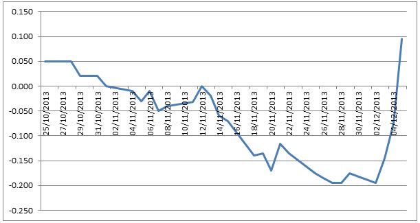
The chart shows the convexity bias that used to exist on Eurodollar futures prior to 2011, when central counterparty clearing for swaps and FRA’s gained traction. Now it has largely disappeared due to the cross margining benefit of both products being cleared and margined by CME Group.
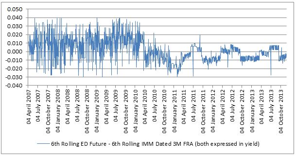
ED Convexity bias
In Europe, the bias went slightly negative this summer mainly since margins for LIFFE Euribor futures could not be netted against margins for Euro FRA’s cleared at SwapClear. Any trader doing the European convexity bias trade would have to post two sets of margin and as the rate paid on margin is lower than the trader’s own funding costs, a substantial funding adjustment results which would be greater than value of the convexity bias. Consequently, there was nothing to prevent the bias going negative!
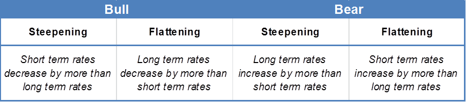
Short term rates and curve steepening or flattening
Many short term rate traders trade the ever changing term structure of rates, called the (yield) curve. Generally, most curve movements can be classified as steepeners (where the differential between long term rates minus short term rates widens) or flatteners (the opposite). They can be further differentiated by bull/ bear steepening/flattening:
One big question remains though – will the curve steepen or flatten? There are many curve drivers but an interesting one is the relationship between short rates like 3-month LIBOR or EURIBOR and steepening or flattening phases.
The chart below shows this relationship for 3-month USD LIBOR (RH scale) and the RedGreen one year Eurodollar calendar spread (LH scale)
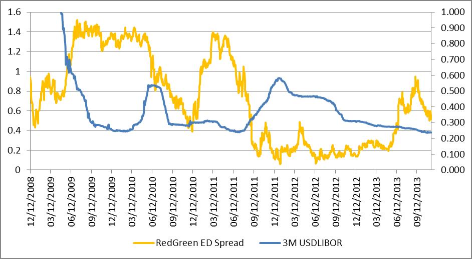
The RedGreen one year Eurodollar calendar spread is the spread between the first red Eurodollar futures and the first green Eurodollar future, rolled every quarterly expiry, expressed in rate terms
(100-Green)-(100-red)
An increase in this spread means the curve is steepening and a decrease means it is flattening.
There is a causal link relationship between the short rate and the state of the curve.
Generally,
- when short rates rise, the curve flattens
- As policy rates increase, pushing money market rates higher, the short end of the curve increases more quickly than the longer end, hence flattening. This is technically a bear flattening.
- And when short rates fall, the curve steepens for the opposite reasons. This is a bull steepening.
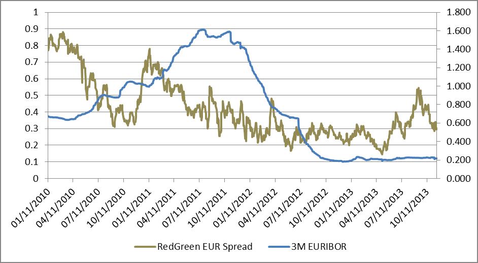
Here’s the same for the Euribor.
Central banks and short rate trending
In the G3 80% of base rate changes are in the same direction as the previous change.
Tapering talk and improved G3 economics leads to one inexorable conclusion: We are probably in the endgame of historically low rates and the consequence of improved economic output and cutbacks in US asset purchase programs should result in steepening yield curves and a general increase in rates.
Although it is unlikely that there will be base rate changes for some time, STIR futures are largely about expectations and the prospect of some eventual central bank action prompted me to revisit an old study from UBS written by Antony Morris called Using trend strategies to benefit from gradualism in monetary policy, October 2006.
This study put forward an interesting hypothesis that central banks create trends in short-term rates and often STIR markets do not price in these trends. Indeed, the table below shows that over a significant period of time, one central bank rates change is followed by one in the same direction.
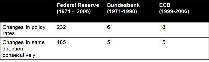
You can’t get much better than that for a long term trending market, something in scarce supply for systematic traders in recent years. Indeed, the trends are actually enforced by the very nature of central banks when compared to other markets like equity.
- Central bankers face few restrictions on timing or tone of their comments on policy compared to that of equity corporate insiders who face considerable restrictions.
- Central Bankers can decide exactly when to make changes at the short end of the curve whereas corporate equity insiders cannot completely control earnings reports
- Central Bankers exercise significant control over the market at the short end,whereas equity corporate insiders cannot control reaction to new new information.
The charts below show these effects. First is the ECB MRO and second Fed Funds both with 9 day and 124 moving averages highlighting the stable long term trends evident in rate cycles.

ECB MRO (black), Euribor front month STIR future 9 day MA (green) Euribor front month STIR future 124 day MA (purple)
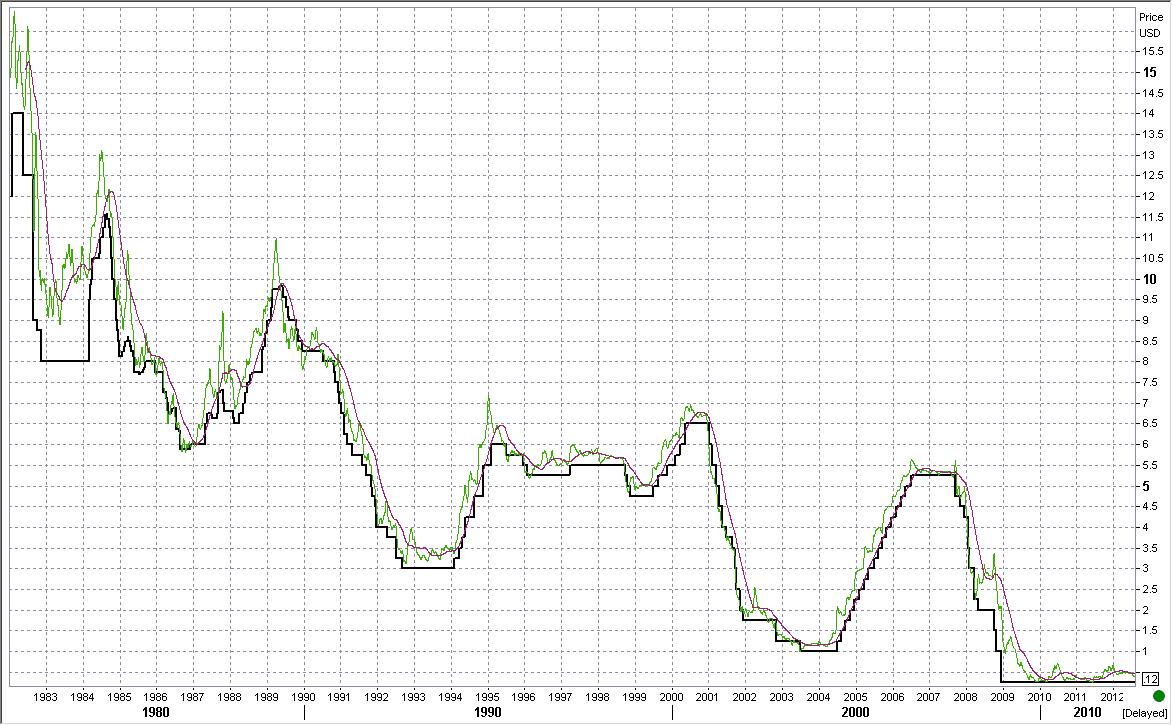
Fed Funds (black), Eurodollar front month STIR future 9 day MA (green) Eurodollar front month STIR future 124 day MA (purple) Both charts from Reuters Eikon.